Dice Simulation in Python
The theory
Dice are thrown to provide random numbers for gambling and other games, and thus are a type of hardware random number generator. The result of a die roll is random in the sense of lacking predictability, not lacking cause. In a fair dice each outcome (side) has the same probability of 1/6.
The implementation it’s easy, all we have to do is create a function in python that returns a random integer between 1 and 6. After that to check if the probabilities of all sides are equal we can repeat this process enough, so we will have a big enough sample size to perform some basic statistics.
The code
First we have to import our necessary libraries to generate our random numbers and visualize the results.
import numpy as np
import matplotlib.pyplot as plt
plt.style.use('classic')
Then we create a function call diceRoll which will generate a random integer between 1 and 6 and return it to us.
def diceRoll():
    return np.random.randint(1,7)
Then we initialize a variable that will store the number of desired rolls, run our experiment and store the results in a list.
number_of_rolls = 10000
results = []
for i in range(number_of_rolls):
    results.append(diceRoll())
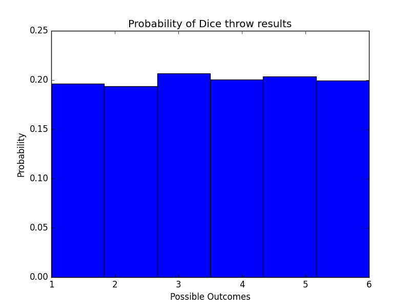
Now we can visualize our results by plotting them using a histogram.
plt.hist(results,density=True,bins = 6)
plt.xlabel("Possible Outcomes")
plt.ylabel("Probability")
plt.title("Probability of Dice throw results")
plt.show()
We choose the number of bins to be 6 because these are our only possible outcomes and we are interested to see how often these appear.
The sum of 2 dice
After seeing the results of a single dice throw, it’s only natural to think how would the probability distribution of the sum of two dice.
Let’s first see some of the theory of two dice throw.
The theory
All possible combinations of two dice throw, our sample space, is
| 1 | 2 | 3 | 4 | 5 | 6 | |
|---|---|---|---|---|---|---|
| 1 | (1,1) | (1,2) | (1,3) | (1,4) | (1,5) | (1,6) |
| 2 | (2,1) | (2,2) | (2,3) | (2,4) | (2,5) | (2,6) |
| 3 | (3,1) | (3,2) | (3,3) | (3,4) | (3,5) | (3,6) |
| 4 | (4,1) | (4,2) | (4,3) | (4,4) | (4,5) | (4,6) |
| 5 | (5,1) | (5,2) | (5,3) | (5,4) | (5,5) | (5,6) |
| 6 | (6,1) | (6,2) | (6,3) | (6,4) | (6,5) | (6,6) |
So as we can see there are 36 possible combinations of rolls and each dice acts independent of the other so to calculate the probability of each pair all we have to do is multiply the probabilities of the individual outcomes and because, as we saw earlier, each individual outcome has a probability of 1/6, each pair of outcomes has a probability of 1/36.
Now for the probability of sum of the two dice we first need to find all the possible outcomes (sums) and all the possible pairs so we can add the probabilities.
| Sum | Possible pairs | Probability |
|---|---|---|
| 2 | 1 | 1/36 |
| 3 | 2 | 2/36 |
| 4 | 3 | 3/36 |
| 5 | 4 | 4/36 |
| 6 | 5 | 5/36 |
| 7 | 6 | 6/36 |
| 8 | 5 | 5/36 |
| 9 | 4 | 4/36 |
| 10 | 3 | 3/36 |
| 11 | 2 | 2/36 |
| 12 | 1 | 1/36 |
Let’s see how we can generate those results and visualize them by reusing the function we wrote for the dice roll.
The code
For these we will use the same function and just call it twice and add the results before we store it to a list. Again we will run this simulation enough times to ensure that we have enough samples to draw a significant conclusion.
results2 = []
for i in range(number_of_rolls):
    results2.append(diceRoll()+diceRoll())
Then we will just plot the histogram to get a better idea of the results.
plt.hist(results2,density=True,bins=11)
plt.xlabel("Possible Outcomes")
plt.ylabel("Probability")
plt.title("Probability of The Sum of Two Dice")
plt.show()
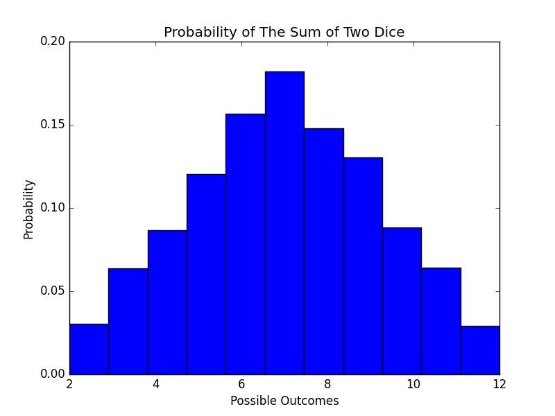
As we can see from the histogram the results of the simulation match the theoretical.
The full code for this article can be found at github