What’s Linear Regression?

Linear regression is a linear model, e.g. a model that assumes a linear relationship between the input variables (x) and the single output variable (y). More specifically, that y can be calculated from a linear combination of the input variables (x).

Let’s consider the model function

y = a + b*x

which describes a line with slope b and y-intercept a. In general such a relationship may not hold exactly for the largely unobserved population of values of the independent and dependent variables; we call the unobserved deviations from the above equation the errors. Suppose we observe n data pairs and call them {(x_i, y_i), i = 1, …, n}. We can describe the underlying relationship between yi and xi involving this error term ε_i by

y_i = a + b * x_i + ε_i. This relationship between the true (but unobserved) underlying parameters a and b and the data points is called a linear regression model.

The goal is to find estimated values for the parameters a and b which would provide the “best” fit in some sense for the data points. The “best” fit will be understood as in the least-squares approach: a line that minimizes the sum of squared residuals. For a better understanding of the theory behind the model you can check here as we won’t get much into it here.

The best estimate for the a parameter is calculated by:

a = (x * y - x * y)/(x^2 - x^2)

and the best estimate for the b parameter is calculated by:

b = y - a * x

The metric we will use to evaluate our results is the value R-Squared. R-Squared is the ratio of the sum of squares regression (SSR) and the sum of squares total (SST). Sum of Squares Regression (SSR) represents the total variation of all the predicted values found on the regression line or plane from the mean value of all the values of response variables. The sum of squares total (SST) represents the total variation of actual values from the mean value of all the values of response variables. R-squared value is used to measure the goodness of fit or best-fit line. The greater the value of R-Squared, the better is the regression model as most of the variation of actual values from the mean value get explained by the regression model.

Let’s see how we can implement that logic with python.

The code

As usual we first import the necessary libraries to perform our calculations and visualizations.

import numpy as np
import matplotlib.pyplot as plt
plt.style.use("classic")

Then, to perform our regression, we need some data points, so lets create a function to generate us that data. The function will take as parameters the number of data points we want to generate, the desired variance, the step we want to move from each data point to the next (this will help us to create positive correlated data points or negative) and the type of correlation we want (if assigned as False we ignore it).

def create_dataset(num_points,variance,step=2,correlation=False):
	val = 1
	ys = []
	for i in range(num_points):
		y = val + np.random.randint(-variance, variance)
		ys.append(y)
		if correlation and correlation=='pos':
			val+=step
		elif correlation and correlation=='neg':
			val-=step

	x = [i for i in range(len(ys))]

	return np.array(x,dtype=np.float64), np.array(ys,dtype=np.float64)

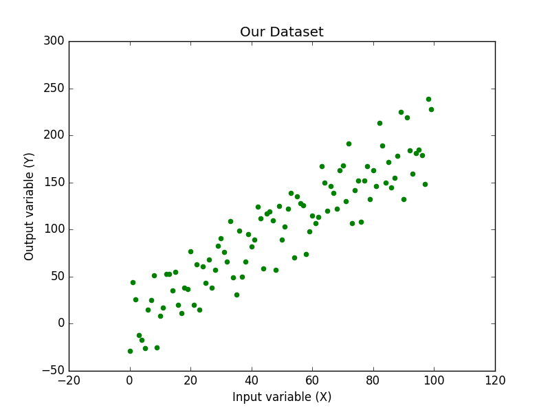
Then to create and visualize our dataset we just call this function to generate our (x,y) pairs and use matplotlib to plot them. Due to the use of random numbers each time we run them we will get slightly different datasets.

xs, ys = create_dataset(100,50,2,correlation='pos') 
plt.scatter(xs,ys,'o')
plt.xlabel("Input variable (X)")
plt.ylabel("Output variable (Y)")
plt.title("Our Dataset")
plt.show()

Then we create the necessary functions to calculate the best values for our parameters a and b, applying the theoretical model.

def best_fit_slope_intercept(x,y):
	a = ( ((np.mean(x)*np.mean(y)) - np.mean(x*y)) /
			((np.mean(x)*np.mean(x)) - np.mean(x*x)))
	b = np.mean(y) - a* np.mean(x)
	return a, b

And finally creating the function to calculate the R-Squared error and the coefficient of determinations so we can see if our results are any good.

def squared_error(y_orig, y_line):
	return np.sum((y_line - y_orig)**2)
		
def coefficient_of_determination(y_orig,y_line):
	y_mean_line = [np.mean(y_orig) for y in y_orig]	
	squared_error_reg = squared_error(y_orig, y_line)
	squared_error_y_mean = squared_error(y_orig, y_mean_line)
	return 1-(squared_error_reg/squared_error_y_mean)

All we have to do now is put all of this together and run our algorithm to generate and visualize the best fit line.

a, b = best_fit_slope_intercept(xs,ys)

regression_line = [(a*x)+b for x in xs]
rsq = coefficient_of_determination(ys,regression_line)

plt.scatter(xs,ys,color="g",label="Data Points")
plt.plot(xs,regression_line,color="r",label="Best Fit line")
plt.title("Linear Regression Results (Best Fit Line)\n R-Squared Error = {}".format(np.round(rsq,3)))
plt.xlabel("Input variable (X)")
plt.ylabel("Output variable (Y)")
plt.legend(loc="best")
plt.show()

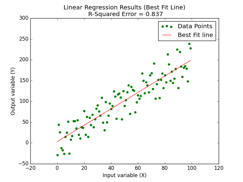
As we can see our R-Squared error is at 0.837 which means we did a pretty good job on our regression.

The full code for this article can be found at github.