Whats is Monte Carlo integration?

In mathematics, Monte Carlo integration is a technique for numerical integration using random numbers. It is a particular Monte Carlo method that numerically computes a definite integral. While other algorithms usually evaluate the integrand at a regular grid, Monte Carlo randomly chooses points at which the integrand is evaluated. This method is particularly useful for higher-dimensional integrals.

So basically to calculate the integral numerically we sample enough random points from our desired interval (a,b), calculate the function at those points take the average and multiply it by the length of the interval (b-a).

To understand this method of numerical integration better we will apply it on 2 different functions one which is one-dimensional (f(x) = sin(x)) and one that is two-dimensional (f(x,y) = cos(x)*exp(y)).

The code

As usual we first import all our libraries.

import matplotlib.pyplot as plt
import numpy as np
from mpl_toolkits.mplot3d import Axes3D
plt.style.use("classic")

Then we have to define any function we want to use.

def func(x):
    return np.sin(x)

def func2d(x,y):
    return np.cos(x)*np.exp(y)

And initialize the number of simulations we want to run as well as the number of random points we want to draw for our function evaluations.

sampling_num = 10000
num_sim = 1000

Before we perform any calculation, we plot our functions in the desired interval, to get a basic idea of what we will be calculating.

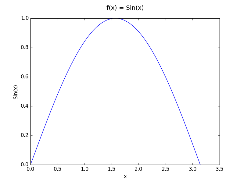
Our first function is the function f(x) = sin(x) in the interval [0,π].

a=0
b=np.pi
x = np.linspace(a,b,sampling_num)
y = func(x)
plt.title("Sin(x)")
plt.xlabel("x")
plt.ylabel("Sin(x)")
plt.plot(x,y)
plt.show()

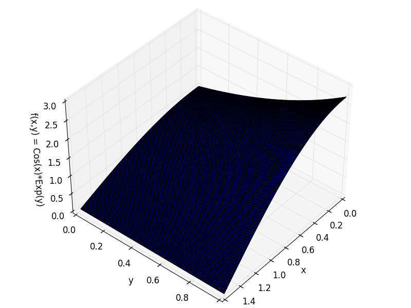
And our 2D function is f(x,y) = cos(x)*exp(y) in [0,π/2]x[0,1].

x_min = 0
x_max = np.pi/2
y_min = 0 
y_max = 1
x = np.linspace(x_min, x_max, sampling_num)
y = np.linspace(y_min,y_max,sampling_num)
X, Y = np.meshgrid(x, y)
func = func2d(X,Y)

fig = plt.figure()
ax = Axes3D(fig)
ax.plot_surface(X, Y, func)
ax.set_xlabel('x')
ax.set_ylabel('y')
ax.set_zlabel('Cos(x)*Exp(y)')
ax.view_init(40,40) 
plt.show()

To visualize our 2D function there are 2 ways. The classical 3D surface plot with axes (x,y,f(x,y)).

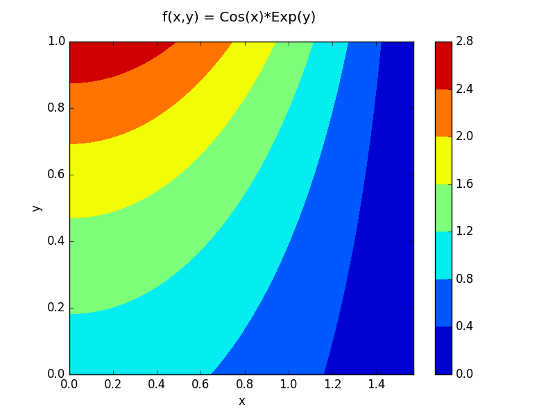
And the contour plot, which is a graphical technique for representing a 3-dimensional surface by plotting constant z slices, called contours, on a 2-dimensional format.

Then we have to define the functions that will perform the integration, for demonstration purposes we define 2 different functions, one for the 1D case and one for the 2D.

def MonteCarloIntegral(function,a,b,sampling_num):
    rest = []
    for n in range(sampling_num):
        rest.append(function(np.random.uniform(a,b)))
    return rest
    
def MonteCarlo2DIntegral(function,x_min,x_max,y_min,y_max,sampling_num):
    rest = []
    for n in range(sampling_num):
        rest.append(function(np.random.uniform(x_min,x_max),np.random.uniform(y_min,y_max)))
    return rest

Then we perform the numerical integration for the first function.

actual_val = 2
err = []
results = []
for i in range(num_sim):
    r = MonteCarloIntegral(sin,b,1,sampling_num)
    integral = (b-a)*np.mean(r)
    results.append(integral)
    err.append(integral-actual_val)
print("Value Calculated = {} ".format(np.mean(results)))
print("Mean error = {}".format(np.mean(err)))

And plot the results in a histogram.

plt.hist(results)
plt.title("Distribution of Areas Calculated")
plt.xlabel("Areas")
plt.ylabel("Number of Times Calculated")
plt.show()

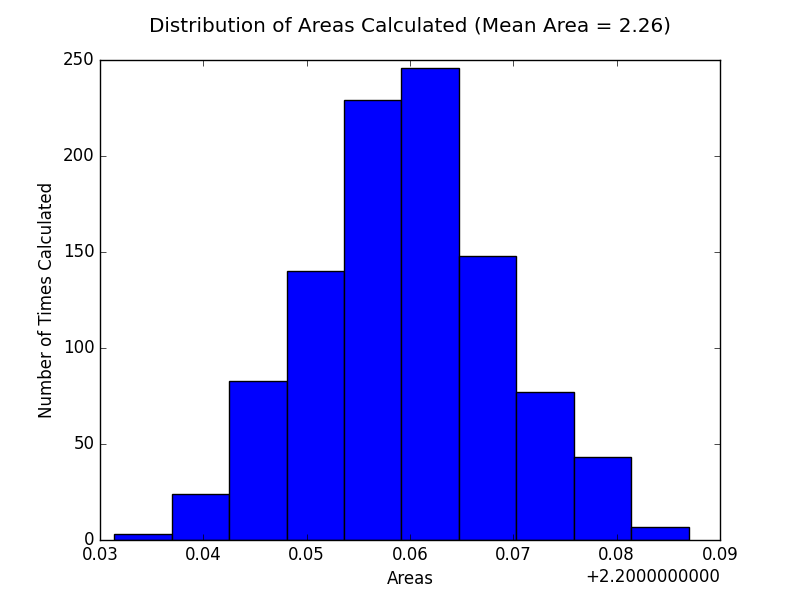
As we can see the analytical solution for the integral is 2 and our numerical solution 2.26, which gives us an error of 0.26. Which means we overestimated by 0.26.

Then we proceed to our 2D function and perform a similar procedure.

actual_value2 = 1.71828
results2 = []
err2 = []
for i in range(num_sim):
    r = MonteCarlo2DIntegral(func2d,x_min,x_max,y_min,y_max,sampling_num)
    integral = (x_max-x_min)*(y_max-y_min)*np.mean(r)
    results2.append(integral)
    err2.append(integral-actual_value2)
print("Value Calculated = {} ".format(np.mean(results2)))
print("Mean error = {}".format(np.mean(err2)))

And we also plot the results in a histogram.

plt.hist(results2)
plt.title("Distribution of Areas Calculated")
plt.xlabel("Areas")
plt.ylabel("Number of Times Calculated")
plt.show()

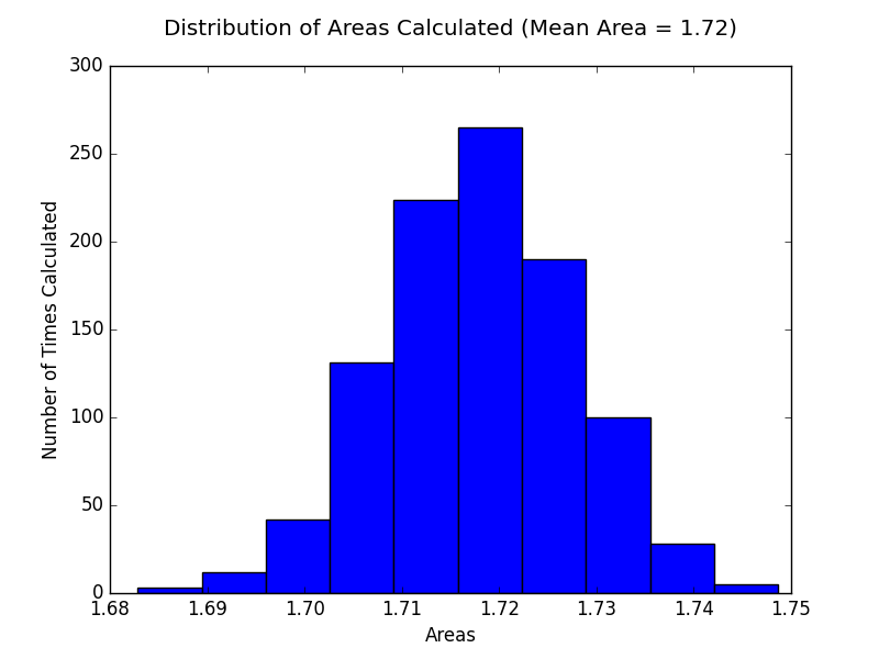
As we can see the analytical solution for the integral is 1.71828 and our numerical solution 1.7177, which gives us an error of -0.00058 . Which means we underestimated by 0.00058.

So as we can see from our results this method works better on higher-dimensional integrals, the theory suggested.

The full code for this article can be found at github.