What is a Monte Carlo Simulation?

Monte Carlo simulation is a technique used to understand the impact of risk and uncertainty in financial, project management, cost, and other forecasting models. A Monte Carlo simulator helps one visualize most or all of the potential outcomes to have a better idea regarding the risk of a decision.

A simple dice game

Lets consider a simple game of dice, each time we roll the dice we bet a certain amount on a certain outcome, if we are correct we win that amount else we lose it.

Lets say each time we bet 1$, our expected profit is 1*(1/6) - 1*(5/6) = -4/6 = -67%. So as we see it’s not wise play this game, but for the sake of this article we will.

So if we start the game with an initial amount of 10000$, decide to roll the dice 100 times and each roll we bet 100$ at the end of the game we expect to lose around on average 67% of our money, which means we should have around 3300$.

Let’s run a Monte Carlo simulation to run different scenarios and visualize our different outcomes.

The code

As always we first need to import any libraries we plan to use. For this example we only need matplotlib and numpy.

import matplotlib.pyplot as plt
import numpy as np
plt.style.use('classic')

Then we will create some functions to help us with the simulation. We need three functions:

1. A function to simulate a dice roll.
2. A function to simulate our player.
3. And a function to run the simulation.

For the dice roll function we can use the one we wrote at Dice Simulation in Python

def diceRoll():
    return np.random.randint(1,7)

For the player function, we will pass as parameters our bet and the result of our dice roll function and if the two match we will return True, else we’ll return False.

def player(bet,dice_result):
    if bet == dice_result:
        return True
    return False

And finally for the simulation function, we will pass as parameters our initial position (10.000$), the number of desired simulations (100), our bet (in the dice example it really doesn’t matter because all outcomes have the same probability), the amount we want to bet at each roll (100$) and the number of bets we want to play for. Then we will loop the number of simulations we passed and at each simulation we will play for the desired number of bets and record our positions after each bet. The function will return a timeseries for each time we run our simulation. Then we can plot them to visualize the results and perform some basic statistics to validate the theoretical results.

def Simulation(initial_position,num_simulations,bet_number,bet_amount,num_of_bets):
    results = []
    for n in range(num_simulations):
        y = [initial_position]
        for i in range(num_of_bets):
            dice = diceRoll()
            if player(diceRoll(),bet):
                y.append(y[-1]+bet_amount)
            else:
                y.append(y[-1]-bet_amount)
        results.append(y)
    return results

We are now ready to initialize our parameters for the simulation and run it.

num_simulations = 1000
initial_position = 10000
num_of_bets = 100
bet_number = 3
bet_amount = 100

results = Simulation(initial_position,num_simulations,bet_number,bet_amount,num_of_bets)

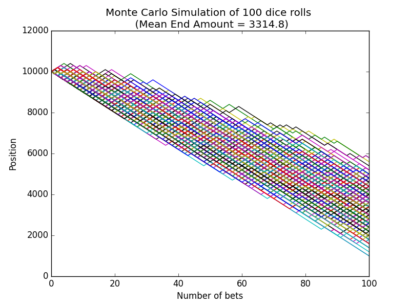
The variable results holds all our timeserieses. By plotting them we can see that our theoretical results match the results of our simulation. As we see each simulation started at 10.000$ and the average amount we have at the end of all the simulations is 3.314,8$ which is around 33.1%.

x = list(range(num_of_bets+1))
end_value = [y[-1] for y in results]
mean_end_value = np.mean(end_value)
for y in results:
    plt.plot(x,y)
    
plt.xlabel("Number of bets")
plt.ylabel("Position")
plt.title("Monte Carlo Simulation of {} dice rolls \n (Mean End Amount = {})".format(num_of_bets,mean_end_value))
plt.show()

Another way to visualize our results is via a histogram.

plt.hist(end_value,density=True)
plt.xlabel("Final amounts")
plt.ylabel("Probability")
plt.title("Histogram of our Final amounts")
plt.show()

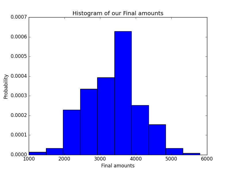
Again, as we see in the histogram, our most common outcome is the 33% loss.

The full code for this article can be found at github.